| ABSTRACT: We analyzed a
new Digital Elevation Model (DEM) of the Putuligayuk watershed,
which flows into Prudhoe Bay, Alaska. We created a new computer-generated
channel-network of this basin and found that the drainage area
is 588 km2 – at least 132 km2 (29%) larger than previously
determined using pre-viously available, less accurate DEMs. Total
lake area was found to be 55 km2, and hypsometry was calcu-lated.
Hydrologic features like thaw lakes, pingos, and river terraces
can also be identified and quantified us-ing this DEM. To our
knowledge, no other DEMs exist of other complete Arctic watersheds
with a comparable accuracy and resolution, thus the advantages
of such DEMs are described. We also discuss how these DEMs can
be used to study the impacts of climate change on Arctic permafrost,
and suggest that an in-ternational Arctic Topographic Mapping
Mission (ATMM) is urgently needed as a baseline to document fu-ture
landscape change.
1 INTRODUCTION
A Digital Elevation Model (DEM) is a mathematical representation
of topography and an indispensable part of most modern terrestrial
research. For exam-ple, DEMs are used as base maps for GIS, hydro-logical
computer models, and data visualization. DEMs are typically distributed
as a matrix of eleva-tion values, where the rows and columns of
the ma-trix represent spatial coordinates, such as latitude and
longitude or UTM Easting and Northing. The term ‘posting’
describes the spatial resolution of a DEM; for example, a DEM
with 100 m posting means that each matrix element represents a
100 m x 100 m area of real ground. Vertical resolution is de-scribed
by the discretization interval – USGS DEM elevations are
available only in integer units of feet, whereas the DEM we analyzed
in this study is in units of centimeters. The smaller the interval
used, the less erroneously-flat areas in the resulting DEM.
DEMs can be created by a variety of techniques, some more accurate
than others for a given resolu-tion. Many DEMs, like those distributed
by the USGS (the only ones commonly available to the public within
the US), are scanned versions of paper topographic maps and are
available with matrix ele-ments of 2 x 3 arc-seconds (roughly
60 m x 90 m) for all of Alaska. Some of the best DEMs created
today are still produced using air photos (skipping the hard copy
step of USGS), with posting down to 1 m. However, these DEMs are
labor intensive to produce, require clear skies, and are typically
very expensive. DEMs based on laser altimetry offer high spatial
resolutions (on the order of centimeters), but again depend on
clear skies and are typically very expensive. Radar systems mounted
on satel-lites, airplanes, and space shuttles have become quite
popular in the past 10 years, and have the advantage of not being
dependant on weather or time-of-day. Resolutions achieved by radar-derived
DEMs are typically not as high as offered by laser altimetry systems,
but the data acquisition is significantly cheaper, especially
when covering large areas.
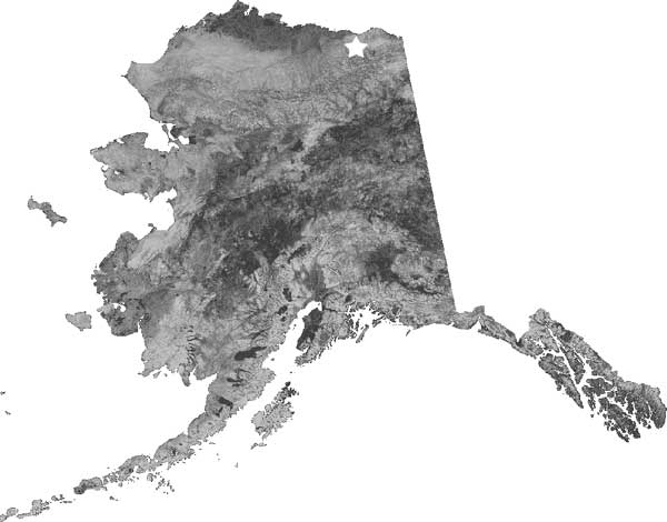
Figure 1: Location map of the Putuligayuk watershed.
Accurate knowledge of terrain is perhaps more important in hydrological
studies in the Arctic than elsewhere, due to the coupling between
the thermal state of the soil and its drainage characteristics.
Be-cause the thermal regime (i.e., active layer depth) has a sensitive
dependence on slope and aspect, the better our knowledge of topography,
the better we can model the coupled thermal and hydrological processes
(Hinzman et al., 1998). This paper pre-sents the results of comparisons
between typical USGS DEMs and a radar-derived Star3i DEM (pro-duced
by Intermap Technologies Corporation in Boulder, CO) for an Arctic
watershed in Alaska, as well as some of the implications of these
compari-sons.
2 RESOLUTION COMPARISON BETWEEN STAR3I
AND USGS DEMS
We were fortunate to obtain and analyze a Star3i DEM of the Putuligayuk
watershed (adjacent to the well-studied Kuparuk watershed) through
funding from NASA (Figure 1). This DEM was delivered with 5 m
postings, 3 m RMS vertical accuracy, and 1 cm vertical resolution
(a more expensive product is also available at 2.5 m posting and
30 cm RMS vertical accuracy). The data was obtained using a LearJet
flying at about 10000 m with an X-band ra-dar interferometry system
acquiring swaths roughly 6 km wide. The data were stitched together
to form a seamless DEM before delivery to us. More de-tailed specifications
can be obtained in their product guide, available through their
website; see Nolan and Fatland (2002) and Nolan et al (2002) for
more information on SAR interferometry and the use of these DEMs
in hydrological application.
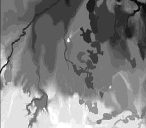 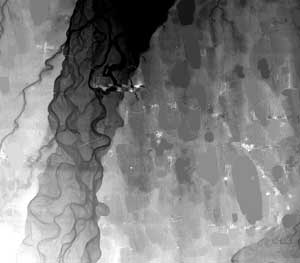
Figure 2A (upper-left), 2B (upper-right), 2C (lower-left), and
2D (lower-right).
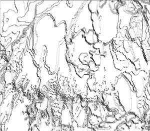 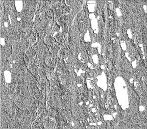
Figure 2. Example resolution comparisons of USGS and Star3i DEMs.
In A and B, darker shades imply lower elevation; an ele-vation
range of 24 m exists within this area. In C and D, white indicates
flat area and shades of gray indicate aspect. The width of each
image is about 17 km. The higher spatial resolution of the Star3i
DEM allows for substantially more topographic detail in B, and
the higher vertical resolution allows features like lakes to be
resolved.
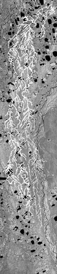 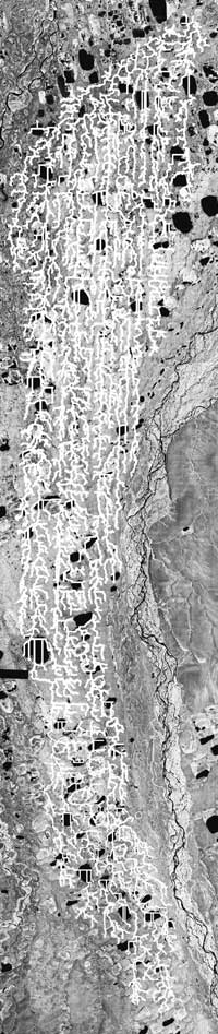 
Figure 3A (left), 3B (middle), 3C (right) - figure 3C not to
scale
Figure 3. Comparison of stream channel networks. In A and B,
thick white lines indi-cate the locations of validated channel
net-works derived from the USGS and Star3i DEMs respectively.
Thin white lines indicate erroneous channel networks that are
pre-dicted by the DEMs to be within the Put wa-tershed, likely
caused by reasons suggested in the text. In C, the gray and black
lines repre-sent the validated watershed boundaries pre-dicted
from the USGS and Star3i DEMs re-spectively. The area predicted
by the Star3i DEM is approximately 25% larger than that from the
USGS DEM. The width of the im-ages at left is 18.5 km.
Although these errors are in general rather minor, they can occasionally
lead to large changes in com-puted watershed size. Figure 3b (arrow)
shows one instance of this that we found in the Putuligayuk DEM.
A small tributary of the Kuparuk crossed a swath-acquisition line,
and was routed south along the seam for only several pixels, which
caused the entire drainage to be ‘diverted’ into the
Putuligayuk watershed. This stream drains an area over 100 km2
to the south, significantly increasing the apparent area of the
Put watershed. While we cannot be defi-nite as to whether or not
this stream changed course or not since the 1950s (when the USGS
air photos were acquired), the close correspondence to the seam
boundary and systematic noise strongly sug-gests it is in error.
These ripples may also cause the channel networks to likely align
more north-south than they are in reality (Figure 3b). However,
there are few actual channels in most of this low-gradient watershed,
so this figure can be somewhat mislead-ing; that is, the computer
algorithm forces every pixel to drain into another, but does not
determine whether or not this drainage occurs through a chan-nel,
overland, or through the vegetative mat. The ef-fects of these
ripples and seem boundaries can be re-duced or eliminated through
smoothing or resampling to a lower resolution. They can also be
eliminated by purchasing the flood plain accuracy Star3i product,
in which a second acquisition of the same area is collected perpendicular
to the first is used to assess and eliminate these errors, at
roughly double the cost.
Thus both DEMs have errors in this low gradient watershed, but
for different reasons. The USGS suf-fers most from poor spatial
and vertical resolution. The Star3i DEM suffers from almost the
opposite problem - because the vertical resolution is so high,
systematic measurement errors on the order of 10 cm can cause
noticeable errors.
4 HYDROLOGICAL ANALYSES
Use of the new Star3i DEM has allowed us to de-termine that the
Put watershed is significantly larger than previously thought.
Figure 3c compares water-shed outlines created with the DEMs.
The USGS DEM yielded a watershed area of 456 km2 ± 3 km2
and the Star3i DEM yielded 588 km2 ± 3 km2 (these figures
do not include area identified as erroneous in the previous section),
for an increase of roughly 29%. Error estimates include only discretization
er-ror and were calculated by dividing the watershed perimeter
by the posting and multiplying by the pixel area. Actual watershed
area is likely larger than the Star3i calculated value, as occasionally
some areas upstream of lakes with multiple inlets were not included
by the program. Visual inspection and calculation of this error
resulted in a maximum area of 10 km2; the possibility exists also
that area we excluded as erroneous (171 km2) should actually be
included, but we consider this unlikely. These areas were calculated
upstream of the USGS gaging station at the bridge near the river
outlet; maximum relief between this location (8 m ASL) is 110
m, spanning a distance of about 65 km.
The hydrological significance of this new water-shed area calculation
is largely related to our ability to calculate an accurate water
balance. Because spa-tial measurement of storage and evaporation
is so difficult, these terms are often estimated as the re-sidual
of the precipitation and river discharge meas-urements per unit
area; that is, Storage+Evaporation = (Precip. – Discharge)/Area.
Therefore, a 29% in-crease in watershed area results in a 29%
decrease in the estimates of storage and evaporation per unit
area. For example the storage estimates from Kane et al., 2001
would change from 24 mm to 30 mm (note that this figure was adjusted
by only 25%, as that research used a watershed area of 471 km2).
Because our best estimates for these terms for the entire Alaskan
Arctic come from the Kuparuk and Put watersheds, the impact of
this difference may be significantly compounded when used in global
cli-mate models. The actual impact has not yet been evaluated
in these models.
Transient water storage in this watershed occurs primarily in
the numerous lakes as well as the tundra itself. Evaporation rates
from lakes are different than from tundra, thus knowing the total
lake surface area is important for partitioning the energy balance.
We found that the total lake surface area contained with the Put
watershed was 55 km2, or 9.3% of the total watershed area, within
a minimum of 1000 total lakes (assessed using the 10 m Star3i
DEM aspect image). This compares well to a minimum saturated area
of about 60 km2 (Kane et al., 2001) determined using satellite
SAR. Lake surface area is also a good starting point for estimating
total lake volume. For example, if we assume that average lake
depth is 3 m (Mellor, 1985), total lake water volume is 0.165
km3.
Figure 4. Hypsometry of the Put watershed. The strong black line
represents total watershed area, while the thin black line represents
the total lake area.
The distribution of area with elevation is shown in Figure 4
for the Put watershed, both for total area and just for lake area.
Such watershed hypsometry is a valuable statistical tool for the
comparison of watersheds. As is clear from this figure, the Put
wa-tershed resides primarily on the low-gradient coastal plains
and foothills, and does not extend into the mountains of the Brooks
Range as does the Kuparuk River.
5 MONITORING SURFACE ELEVATION TO
DETECT CLIMATE CHANGE
Though we have shown that improved DEMs will yield improved quantification
of hydrologic vari-ables such as watershed areas and stream channels,
the level of improvement in this case allows for the detection
of future topographic change in the Arctic in ways previously
impossible. For example, the ac-curacy and resolution of these
DEMs are sufficient to identify pingos and calculate their size
and shape using computerized algorithms (Figure 5a), such that
change detection can be measured using DEMs cre-ated in the future.
Because the steep south-facing slopes of pingos harbor vegetative
islands, the dy-namics of these communities in relation to climate
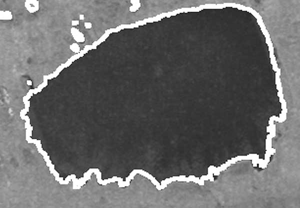
change can be modeled with increased accuracy. Lake boundaries
can be measured accurately enough such that boundary migration
can be measured on the time-scale of 5 years, assuming a minimum
migration rate of 25 cm a-1, as has been observed in some areas;
Figure 5b compares a lake outline derived from the Star3i data
compared to an airphoto acquired in 1972. Thermokarsting and subsidence
can be measured over enormous areas with a resolu-tion of centimeters;
much of this activity might oth-erwise go unnoticed and would
certainly be impos-sible to characterize with anywhere near the
clarity using ground-based surveying. Coastal erosion in the Arctic
is well known to be widespread and mas-sive in scale (meters per
year), but measurements are isolated to a few areas; repeated
DEM measurements can quantify these erosion rates accurately and
be used to identify variations in rate better than perhaps any
other method (e.g., surveying or optical im-agery). DEMs of this
accuracy have also recently been shown to be the key to making
measurements of soil moisture from space (Nolan and Fatland, 2002;
Nolan et al, 2002). NASA has recently fin-ished its Space-shuttle
Radar Topography Mission (SRTM), which created a DEM of the entire
planet between about +60º and –50º (missing the
Arctic), as well as its Antarctic Mapping Mission (AMM). What
is needed now is an Arctic Topographic Map-ping Mission (ATMM)
before more landscape changes occur, to establish a baseline for
future change detection. To our knowledge, no such effort is planned.
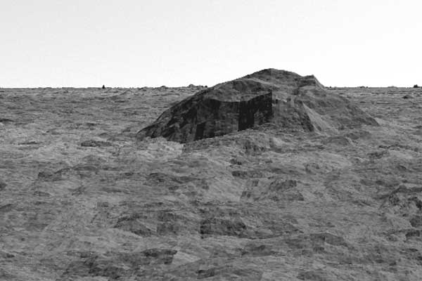
Figure 5A (top), 5B (bottom)
ACKNOWLEDGEMENTS
The Star3i DEM used in this analysis was funded by the NASA Commercial
Remote Sensing Program and analysis funded in part by Grant OPP-0207220
National Science Founda-tion and a grant from the International
Arctic Research Consortium (IARC). Any opinions, findings, and
conclu-sions or recommendations expressed in this material are
those of the author(s) and do not necessarily reflect the views
of the NSF, NASA, or IARC.
REFERENCES
Hinzman, Larry, Doug Goering, and Doug Kane, 1998. A distributed
thermal model for calculating soil temperature profiles and depth
of thaw in permafrost regions. JGR, Vol 103(D22), 28975-28991.
Kane, Douglas, Laura Bowling, Robert Gieck, Larry Hinzman, and
Dennis Lettenmaier, 2001. The role of surface storage in a low-gradient
Arctic watershed. Northern Research Ba-sins 13th International
Symposium and Workshop, August 19-24, 2001.
Mellor, J.C, 1985. Radar-interpreted Arctic Lake Depths. BLM-Alaska
Open File Report PT 85-020-7200-029.
Nolan, Matt and Dennis R. Fatland, 2002. Penetration depth as
a DInSAR observable and proxy for soil moisture. IEEE TGRS, in
press.
Nolan, Matt, Dennis R. Fatland, and Larry Hinzman, 2002. DInSAR
measurement of soil moisture. IEEE TGRS, sub-mitted.
|
